While working on deep learning, we all have come across the term ‘Convolutional neural network’ or CNN, but what this convolution actually mean. This is a method, operation, rule, instruction or algorithm which we know in this article. So convolution is a mathematical operation and the term ‘Convolutional neural network’ indicates that the network employs a mathematical operation called convolution. Convolution is a specialized kind of linear operation. Convolution is an operation on two functions of a real-valued argument that produces a third function. The term convolution refers to both the result function and to the process of computing it. It is defined as the integral of the product of the two functions after one is reflected about one of the axes and shifted. The integral evaluated for all values of shift, producing the convolution function.

In convolutional network terminology, the first argument (say f here) to the convolution is often referred to as the input and the second argument (g here) as the kernel. The output is sometimes referred to as the feature map.

Let s(t) be the convolution operation with x and w as input and kernel respectively.

If we use two dimensional tensor as our input (tensor is described in this article), we probably want to use a two-dimensional kernel K.
Convolution is a commutative mathematical operation, so we can write it as:

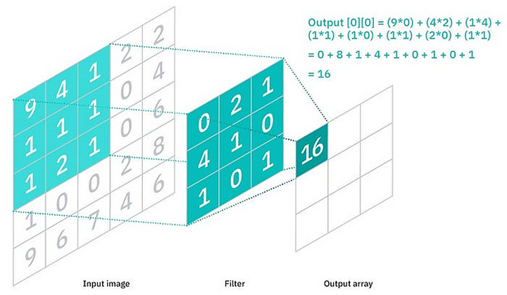
Let us see an example of 2D convolution

Let us see how convolution operation takes place with input map and kernel.

Let us define different parameters of convolutional layer.

Kernel size: It defines the field of view of convolution
Stride: It defines the step size of the kernel when traversing the tensor
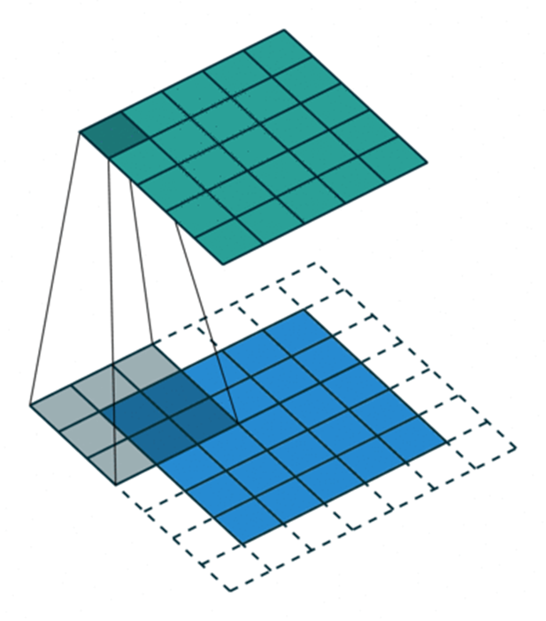
Padding: It defines how the border of a sample is handled.
Input and Output channels: It takes a certain number of input and calculates specific number of output channels.
Let us see different types of convolution
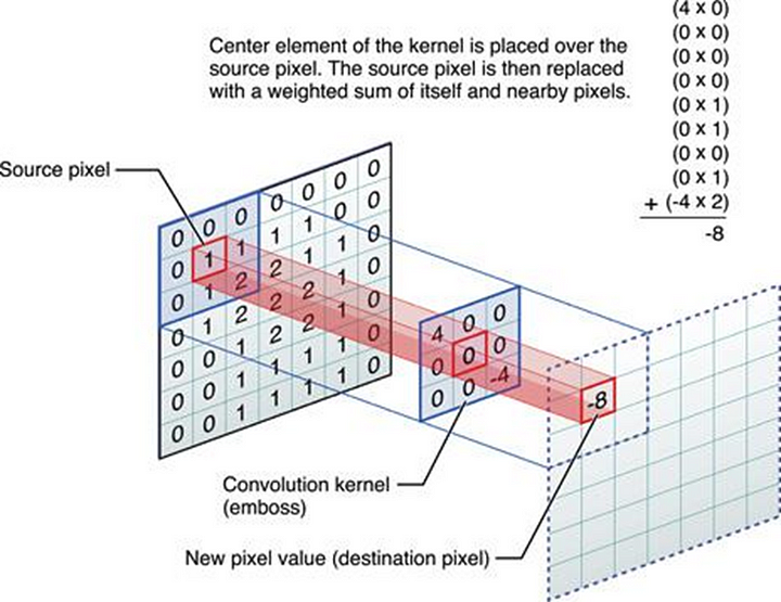
Simple Convolution
This is just a simple convolution operation with a kernel filter that is placed over input map and traverse. Center element of the kernel is placed over the source pixel. The source pixel is then placed with a weighted sum of itself and nearby pixels.

import torch
import torch.nn.functional as F

# With square kernels and equal stride
filters = torch.randn(8, 4, 3, 3)
inputs = torch.randn(1, 4, 5, 5)
F.conv2d(inputs, filters, padding=1)
Applies a 2D convolution over an input image composed of several input planes.
Pointwise Convolution
This is a type of convolution that uses a 1x1 kernel which iterates through every single point. This type of convolution has application that it helps in changing the depth of the input channel without changing its other dimension.

There are two ways to perform pointwise convolution as it is just a linear operation too. Let us see both of them.
1. Using Conv2d
We will take Conv2d and kernel size as 1x1 here.
import torch
import torch.nn as nn

batch_size = 10
channels = 64
h, w = 128, 128
x = torch.randn(batch_size, channels, h, w)
Conv = nn.Conv2d(64, 1, 1, bias=False)
Output_conv = conv(x)
2. Using Linear
import torch
import torch.nn as nn

batch_size = 10
channels = 64
h, w = 128, 128
x = torch.randn(batch_size, channels, h, w)
lin = nn.Linear(64, 1, bias=False)
With torch.no_grad():
  lin.weight = nn.Parameter(conv.weight.view(1, channels))
output_lin = lin(x.view(batch_size, channels, -1).transpose(-2, -1)).transpose(-1, -2)
output_lin = output_lin.view(batch_size, 1, h, w)
Separable Convolution
This is a convolution which can be separated into two convolutions. In regular convolution, if we have a kernel with size 3x3 then we directly apply this over the input map and perform convolution. So based on the separation, we have 2 types of separable convolutions:
1. Spatially separable convolution
In this convolution, we separated the kernel size such that one of the dimension becomes 1. For example, if we have a kernel of size 3x3 then we first perform convolution with kernel of size 3x1 and then with kernel of size 1x3. If we calculate the number of parameters here, we find that we need only 6 parameters in this method while 9 parameters in regular convolution. So it is useful as it is parameter efficient.

We can perform spatial separable convolution by taking convolution two times as
import torch
import torch.nn.functional as F

input_tensor = torch.randn(1, 1, 64, 64)
kernel_row = torch.randn(1, 1, 1, 3) # 1 input channel, 1 output channel, 1x3 kernel
kernel_col = torch.randn(1, 1, 3, 1) # 1 input channel, 1 output channel, 3x1 kernel
# Apply the row convolution
row_conv = F.conv2d(input_tensor, kernel_row, padding=(0, 1))
# Apply the column convolution
col_conv = F.conv2d(row_conv, kernel_col, padding=(1, 0))
2. Depthwise Separable Convolution
In this type of separable convolution, we separate input map as well as kernel in different channels and then apply a single convolutional filter for each input channel. The depth of the filter is same as the input in regular convolution and we mix channels to generate each element in the output while in depthwise, we separately perform convolution for each channel and then stack them.

import torch
import torch.nn as nn

input_tensor = torch.randn(1, 3, 64, 64) # Batch size of 1, 3 channels, 64x64 image
# Define the depthwise convolution layer
depthwise_conv = nn.Conv2d(in_channels=3, out_channels=3, kernel_size=3, padding=1, groups=3)
# Apply the depthwise convolution
output = depthwise_conv(input_tensor)
print(output.shape)
Here When groups == in_channels and out_channels == K \ in_channels, where K* is a positive integer, this operation is known as a “depthwise convolution”
Grouped Convolution
This type of convolution uses a group of convolutions that is multiple kernels per layer which results in multiple channel outputs per layer. This leads to get help to a network learn a varied set of low level and high level features from wider networks.

import torch
import torch.nn as nn

input_tensor = torch.randn(1, 4, 10, 10)
nn.Conv2d(in_channels=4, out_channels=8, kernel_size=3, groups=2)
Shuffled Grouped Convolution
Shuffled Grouped convolution is a type of convolution which is a combination of two techniques that are grouped convolution and channel shuffle. After performing grouped convolution, the channels are shuffled to ensure that information is shared across different groups. In this way, we can preserve the computational benefits of grouped convolutions and also maintain the representational power of network. It will also improve the network’s ability to learn complex features.

import torch
import torch.nn as nn

input_tensor = torch.randn(1, 16, 32, 32)
batch_size = 1
in_channels = 16
out_channels = 32
kernel_size = 3
groups = 4
height = 32
width = 32
batch_size, num_channels, height, width = input_tensor.size()
group_conv = nn.Conv2d(in_channels, out_channels, kernel_size, groups=groups)
x = group_conv(x)
# Reshape to (batch_size, groups, out_channels // groups, height, width
x = x.view(batch_size, groups, -1, height, width)
# Transpose to (batch_size, out_channels // groups, groups, height, width)
x = x.transpose(1, 2).contiguous()
# Reshape back to (batch_size, out_channels, height, width)
x = x.view(batch_size, -1, height, width) #Batch size of 1, 16 input channels, 32x32 image
Transposed Convolution
Transposed convolution, also known as deconvolution or fractionally-strided convolution, is a technique used in convolutional neural networks (CNNs) to increase the spatial resolution of the input feature map. Unlike standard convolution, which reduces the spatial dimensions, transposed convolution expands them. This makes it particularly useful in tasks like image segmentation and generative models where upsampling is required.
Here the filter slides over the input, but instead of reducing the size, it increases it by inserting zeros between the elements of the input tensor and then applying the convolution operation.

import torch
import torch.nn.functional as F

# Define input tensor
input_tensor = torch.randn(1, 3, 32, 32) # Batch size of 1, 3 input channels, 32x32 image
# Define transposed convolution parameters
in_channels = 3
out_channels = 6
kernel_size = 3
stride = 2
padding = 1
output_padding = 1
# Define weights for the transposed convolution
weights = torch.randn(in_channels, out_channels, kernel_size, kernel_size)
# Apply transposed convolution
output = F.conv_transpose2d(input_tensor, weights, stride=stride, padding=padding, output_padding=output_padding)
print(output.shape) # Should be (1, 6, 64, 64)
Dilated Convolution
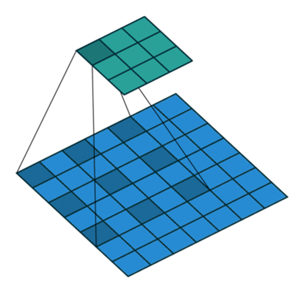
Dilated convolution, also known as atrous convolution, is a technique used in convolutional neural networks (CNNs) to increase the receptive field of the convolutional layer without increasing the number of parameters. This is achieved by inserting zeros between the elements of convolutional kernel. In a standard convolution, the filter slides over the input feature map and computes the dot product. In dilated convolution, the filter is “dilated” by inserting gaps between the filter values. The dilation rate determines the size of these gaps.

import torch
import torch.nn.functional as F

# Define input tensor
input_tensor = torch.randn(1, 3, 32, 32) # Batch size of 1, 3 input channels, 32x32 image
# Define dilated convolution parameters
in_channels = 3
out_channels = 6
kernel_size = 3
stride = 1
padding = 2
dilation = 2
# Define weights for the dilated convolution
weights = torch.randn(out_channels, in_channels, kernel_size, kernel_size)
# Apply dilated convolution
output = F.conv2d(input_tensor, weights, stride=stride, padding=padding, dilation=dilation)
print(output.shape) # Should be (1, 6, 32, 32)
Flattened Convolution
Flattened convolution is a technique designed to accelerate the feedforward execution of convolutional neural networks (CNNs) by reducing the redundancy of parameters. This method involves using one-dimensional filters across different directions in 3D space, instead of the traditional 3D filters used in standard convolutions. In a standard convolution, a 3D filter slides over the input feature map to perform the convolution operation. In flattened convolution, the 3D filter is decomposed into a sequence of 1D filters that perform convolutions across different dimensions (height, width, and depth) separately. This reduces the number of parameters and computational complexity while maintaining performance.

import torch
import torch.nn.functional as F

# Define input tensor
input_tensor = torch.randn(1, 3, 32, 32) # Batch size of 1, 3 input channels, 32x32 image
# Define flattened convolution parameters
in_channels = 3
out_channels = 6
kernel_size = 3
stride = 1
padding = 1
# Define weights for the flattened convolution
weights_h = torch.randn(out_channels, in_channels, kernel_size, 1) # Horizontal filter
weights_w = torch.randn(out_channels, in_channels, 1, kernel_size) # Vertical filter
# Apply horizontal convolution
output_h = F.conv2d(input_tensor, weights_h, stride=stride, padding=padding)
# Apply vertical convolution
output_w = F.conv2d(input_tensor, weights_w, stride=stride, padding=padding)
# Combine the results
output = output_h + output_w
print(output.shape) # Should be (1, 6, 32, 32)
We have seen different types of convolution, what convolution actually is, how to code for all convolution types.
That’s it in this article.
Thanks!
— Akhil Soni
