
This article tells the classification aspect of support vector machines. Support vector machines are very powerful machine learning model. They have the capability to perform linear as well as non-linear classification, regression and they are effective for outlier detection. SVMs are well suited for classification problems in which they are used to classify two classes which are also separable.
Specialization in the category of classication -
For complex datasets
Small or medium datasets
SVM is a type of machine learning algorithm that finds the optimal decision boundary (hyperplane) between two classes of data while maximizing the margin between the classes. Though they are used for classification of both linear and non-linear data.
In this article, we will cover the concept of linear SVM classification.
Linear SVM Classification
As we have already seen in previous articles, there are many other ML models and algorithms which are used for linear classification such as logistic regression, SGD classifier, Lasso and Ridge classifier. One of the most effective classifier is SVM that is support vector machine.
Before getting into it, let us know what are linearly separable classes.
Linearly separable classes — Linearly separable classes or data are a type of binary classification problem in which two classes, one positive and one negative can be separated by a decision boundary. Decision boundary is a boundary that is a linear function of the features of the data given that separates the classes.

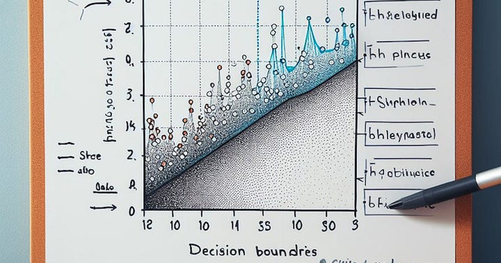
This is a graph showing linearly separable classes. There are three different decision boundaries but if we clearly observe then red and green boundaries are so close to the data points that these models may not perform well on new instances added to the data. We can think that black line shows the boundary made by SVM. SVMs are very effective in such cases and they prepare good decision boundaries with proper margins for both classes. The margin is the distance between the decision boundary and the nearest data points from each class. SVM always try to increase this decision boundary as much as possible so that the distribution remains same for both and they would not produce any error and perform better even if new data instances are added to the data.
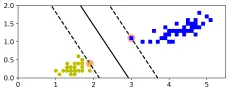
The graph shown above shows the decision boundary prepared by SVM for the data points. The dotted lines show the margins for both classes.
Large Margin Classification
Large Margin refers to the wide separation or “margin” between the decision boundary (hyperplane) and the nearest data points of each class.
In a large margin classification, the SVM tries to find a decision boundary that not only correctly classifies the data points but also maximizes the margin between the classes.
It provides an effective classification for newly added instances and fewer outliers in classification.
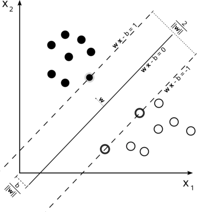
Adding more instances “off the street” will not affect the decision boundary at all; it is fully determined by the instances located on the edge of the street. These instances are called the support vectors.
Hard Margin Classification and Soft Margin Classification
Hard margin classification is a type of SVM classification in which the SVM aims to find a decision boundary (hyperplane) that perfectly separates the data into two classes without any misclassifications. If we strictly impose that all instances be off the street and on the right side, this is called hard margin classification.
There are two main issues with hard margin classification.
1. It only works if the data is linearly separable
2. It is quite sensitive to outliers
It is advised to use flexible model. The objective is to find a good balance between keeping the street as large as possible and limiting the margin violations. This is called soft margin classification.
In soft margin classification, the SVM allows for some misclassifications, and the goal is to find a decision boundary that still maximizes the margin but tolerates a certain amount of classification errors. This approach is used when the data is not perfectly separable due to overlapping points or outliers. Trying to achieve a hard margin in such cases might result in an overly complex and sensitive model.
In scikit-learn’s SVM classes, this balance can be controlled by C hyperparameter. A low C value leads to large margin but many instances end up on the street. A high C values makes fewer margin violations but ends up with smaller margin.
Note — If SVM is overfitting, it can be regularized by reducing C.
There are two SVM classes for classification:
1. LinearSVC with C and loss
2. SVC with kernel and C
SGDClassifier can also be used with alpha=1/(m*C)
SVC is very slow, especially with large datasets, so not recommended.
The LinearSVC class regularizes the bias term, so center the training set first by subtracting its mean or use StandardScaler to scale it. Make sure to use hinge as loss as it is not default. Finally, set dual hyperparameter to False.
Methods
Predict confidence scores for samples.
densify()
Convert coefficient matrix to dense array format.
fit(X, y[, sample_weight])
Fit the model according to the given training data.
Get metadata routing of this object.
get_params([deep])
Get parameters for this estimator.
predict(X)
Predict class labels for samples in X.
score(X, y[, sample_weight])
Return the mean accuracy on the given test data and labels.
set_fit_request(*[, sample_weight])
Request metadata passed to the fit method.
set_params(**params)
Set the parameters of this estimator.
set_score_request(*[, sample_weight])
Request metadata passed to the score method.
sparsify()
Convert coefficient matrix to sparse format.
Given is a code for linear classification using LinearSVC.
import numpy as np
from sklearn import datasets
from sklearn.pipeline import Pipeline
from sklearn.preprocessing import StandardScaler
from sklearn.svm import LinearSVC

iris = datasets.load_iris()
X = iris["data"][:, (2, 3)]
y = (iris["target"] == 2)

svm_clf = Pipeline([
    ("scaler", StandardScaler()),
    ("linear_svc", LinearSVC(C=1, loss="hinge"))
])
svm_clf.fit(X, y)

svm_clf.predict([[5.5, 1.7]])
The above code is written to separate the class for Iris-virginica from all other classes. Here, we have used LinearSVC class with C=1 and loss set to hinge. The SVM classification code can also be written with SVC class with kernel=“linear” and C=1.
import numpy as np
from sklearn import datasets
from sklearn.pipeline import Pipeline
from sklearn.preprocessing import StandardScaler
from sklearn.svm import SVC

iris = datasets.load_iris()
X = iris["data"][:, (2, 3)]
y = (iris["target"] == 2)

svm_clf = Pipeline([
    ("scaler", StandardScaler()),
    ("linear_svc", SVC(kernel="linear", C=1))
])
svm_clf.fit(X, y)

svm_clf.predict([[5.5, 1.7]])
The above code is written with SVC class in which the kernel set to “linear” so that it can also act as LinearSVC but it is slow, especially with large training sets, so it is not recommended.
Methods
Evaluate the decision function for the samples in X.
fit(X, y[, sample_weight])
Fit the SVM model according to the given training data.
Get metadata routing of this object.
get_params([deep])
Get parameters for this estimator.
predict(X)
Perform classification on samples in X.
Compute log probabilities of possible outcomes for samples in X.
Compute probabilities of possible outcomes for samples in X.
score(X, y[, sample_weight])
Return the mean accuracy on the given test data and labels.
set_fit_request(*[, sample_weight])
Request metadata passed to the fit method.
set_params(**params)
Set the parameters of this estimator.
set_score_request(*[, sample_weight])
Request metadata passed to the score method.
Another option is to use the SGDClassifier class, with SGDClassifier(loss=”hinge”, alpha=1/(m*C)). This applies regular Stochastic Gradient Descent to train a linear SVM classifier. It does not converge as fast as the LinearSVC class, but it can be useful to handle huge datasets that do not fit in memory (out-of-core training), or to handle online classification tasks.
That's all in this article.
Thank you!
- Akhil Soni