In the article named “Convolution in NN”, just as we have seen that convolutional networks can process images of variable size, can readily scale to images with large width and height, we are also having the networks that can scale much longer sequences that would be practical for networks without sequence based specialization, these networks are called recurrent neural networks. These networks can also process sequences of variable length.
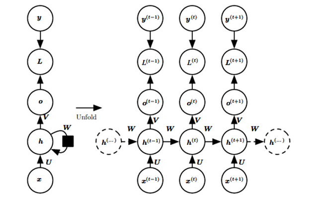
A simple form of RNN can be created by connecting the outputs from a fully connected layer to the inputs of that same layer. The number of inputs to a neuron in an RNN layer is dependent both on the number of inputs to the layer and the number of neurons in the layer itself. For simplicity of exposition, we refer to RNNs as operating on a sequence that contains vectors x(t) with the time step index t ranging from 1 to τ. Let’s see the recurrent network with computational graphs. A computational graph is a way to formalize the structure of a set of computations, such as those involved in mapping inputs and parameters to outputs and loss.
Let’s see about unfolding computational graphs. The idea of unfolding a recursive or recurrent computation into a computational graph that has a repetitive structure, typically corresponding to a chain of events is described here.
Consider the classical form of a dynamical system:

Where s^(t) is called the state of the system.
This equation is a recurrent equation because the definition of s at time t refers back to the same definition at time t-1.
For τ = 3 time steps, the graph can be unfolded as

Such an expression can be represented by a traditional directed acyclic computational graph.

The classical dynamical system described in the equation is now illustrated in the form of an unfolded computational graph. Here each node represents the state at some time t and the function f maps the state at t to state at t+1.
Here when there is an external signal x(t) which can be anything as a parameter to be used driving this recurrent function, the network typically learns to produce state h(t) as a kind of lossy summary of the task relevant aspects of the past sequence of inputs up to t. The unfolded recurrence after t steps with a function g(t) can also be represented as

The function g(t) takes the whole past sequence as input and produces the current state, but the unfolded recurrent structure allows us to factorize g(t) into repeated application of a function f.
Adding the beauty of graph unrolling and parameter sharing, we can design a wide variety of recurrent neural networks.

Let’s see the mathematical representation of a recurrent layer
We know that a fully connected layer can be represented mathematically by multiplying the input vector by a vector matrix, where each row in the matrix represents the weights for a single neuron. With a tanh activation function this can be written as follows:
y = tanh(Wx) where the x is input vector and W is the weight vector.
Here we have taken activation function as tanh. Let’s add bias vector b having same number of elements as number of neurons to the input of this activation function.
y = tanh(Wx+b)
From the figure, we can find that

As here the h^(t-1) arrived from the previous input and x^(t) is the new input here. So the new hidden layer is the combination of previous layer hidden which is again the combination of previous input with its previous hidden layer and the new input. So the new layer is also getting the information from previous input too which is making the model to learn to predict new output learning the pattern from previous outputs. It is the fact that learning from past helps in getting output for present. Here U and W are weight matrices for input to hidden and hidden to hidden connections with parameters as bias vector b.

Now output will be derived as normal linear equation which is the linear layer as discussed in this article.

where V is the weight matrix from hidden to output and c is the bias for this linear layer and final output will be given as

Let us see an example how RNNs work and recognize patterns in sequences of data, such as time series or text. Here we will use RNN to predict the next value in a series of numbers, we will build a basic synthetic dataset.
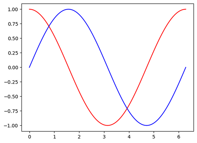
In this example, data shows a nonlinear cyclical pattern between input and output.
x_np = np.sin(steps) #blue
y_np = np.cos(steps) #red

Let us not build an RNN model
class RNN(nn.Module):
  def __init__(self):
    super(RNN, self).__init__()
    self.rnn = nn.RNN(
        input_size = INPUT_SIZE, hidden_size=32,
        num_layers = 1, batch_first = True
    )
    self.out = nn.Linear(32, 1)

  def forward(self, x, h_state):
    r_out, h_state = self.rnn(x, h_state)
    outs = []
    for time_step in range(r_out.size(1)):
      outs.append(self.out(r_out[:, time_step, :]))
    return torch.stack(outs, dim=1), h_state
We will use mse loss and adam optimizer here
for step in range(60):
  start, end = step*np.pi, (step+1)*np.pi
  steps = np.linspace(start, end, TIME_STEP, dtype=np.float32)
  x_np = np.sin(steps)
  y_np = np.cos(steps)
  x = Variable(torch.from_numpy(x_np[np.newaxis, :, np.newaxis]))
  y = Variable(torch.from_numpy(y_np[np.newaxis, :, np.newaxis]))
  prediction, h_state = rnn(x, h_state)
  h_state = Variable(h_state.data)

  loss = loss_func(prediction, y)
  optimizer.zero_grad()
  loss.backward()
  optimizer.step()


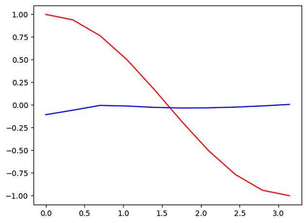
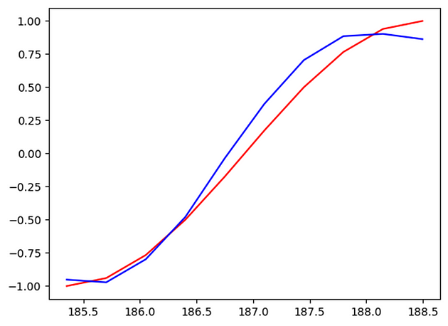
Here red is showing the actual output while blue is the predicted output and that too with epochs = 60. Here we are using sine values as input and cosine as output. So we can observe how RNN is learning to predict new values of cosine learning the previous values of input from sine and then using new sine input value to predict the cosine value for new input.
One of the first recurrent networks that we are aware of is the Hopfield network (Hopfield, 1982). Finally, it is worth saying that an RNN will learn to identify patterns in a sequence irrespective of where in the sequence it appears. This is beneficial because many sequences do not necessarily have a specific starting point, but we choose to start sampling at an arbitrary timestep.
That’s it in this article
Thanks!
Keep exploring more…
— Akhil Soni