In one of my articles, I have already discussed training of a linear regression model. Training a model means setting its parameters so that the model best fits the training set. Best fitting the training set means that the performance measure cost function for the model must be minimum.

In this article, we will know about the training of the logistic regression models.

Logistic Regression

Logistic Regression is commonly used to estimate the probability that an instance belongs to a particular class. If the estimated probability is greater than 50% for a class then, it would classify the data belongs to that class. Let us see how we can estimate the probabilities for classes.

Estimating Probabilities

Here we have the equation to calculate the probability of the logistic regression model:

$$\hat{p} = h_{\theta} (x) = \sigma (x^{T}\theta)$$

where x is the feature vector

θ is the parameters vector

and σ(.) - is a sigmoid function that outputs a number between 0 and 1.

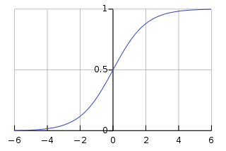
Logistic function:

$$\sigma (t) = \frac{1}{1 + exp(-t)}$$

Logistic function is just same as sigmoid function. Sigmoid function is having its domain as all the real numbers and its range (0, 1). From the value of x^T θ, we have a real value which can act as argument for the sigmoid function or logistic function which will calculate as per the equation of σ(t) and output a number between 0 and 1, with which one can get the probability for the class of logistic regression model. The class for which the probability is greater than 50%, its output will be 1. While if the probabiliy is less than 50%, the output will be 0.

Here the prediction for the logistic regression model can be given by:

$$\hat{y} = \mathrm{\{}_{0,\ \text{if} \ \hat{p} \ \lt \ 0.5 }^{1,\ \text{if} \ \ \hat{p} \ \ge \ 0.5}$$

We can clearly notice it in the graph of logistic function that when the argument value t is less than 0 then value of σ(t) is less than 0.5 and when the value of t is greater than or equal to 0, the value of σ(t) is greater than or equal to 0.5. So, a logistic regression model predicts 1 if x^T θ is positive and 0 if x^T θ is negative as

$$\hat{y} = \mathrm{\{}_{0,\ \text{if} \ x^{T}θ \ \lt \ 0 }^{1,\ \text{if} \ \ x^{T}θ \ \ge \ 0}$$

Training logistic Regression model

We need to set the parameter vector in such a way that it minimizes the cost function which is the performance measure for the models to minima.

Logistic Regression cost function for a single training instance:

$$c(\theta) = \mathrm{\{}_{-log(\hat{p}) \ if\ y\ =\ 1 }^{-log(1-\hat{p})\ if\ y\ =\ 0}$$

This cost function makes sense because as t approaches 0, -log(t) grows very large, so cost will be large and probability will be close to 0 for positive instance.

The cost function for the complete training set is simply the average of all the training instances over all the training data sets. It can be simply called as log loss.

Logistic Regression cost function (log loss):

$$J(\theta) = -\frac{1}{m} \sum_{i=1}^{m} [y^{(i)}log(\hat{p}^{(i)})+(1-y^{(i)})log(1-\hat{p}^{(i)}) ]$$

The bad news is that it does not have any closed-form solution to train the model and set the parameters directly that minimizes the cost function. A gradient descent algorithm can be used to find the optimum solution that gives a global minimum as it is a convex function.

Logistic cost function partial derivatives:

$$\frac{\partial J(\theta)}{\partial \theta_{j}} = \frac{1}{m} \sum_{i=1}^{m} [\sigma(\theta^{T}{x}^{(i)})-y^{(i)} ]x_{j}^{(i)}$$

Once we get the partial derivatives, we can perform any gradient descent algorithm and can train the model easily.

from sklearn import datasets
from sklearn.linear_model import LogisticRegression
import numpy as np

iris = datasets.load_iris()
X = iris["data"][:, 3:]
y = (iris["target"]==2).astype(np.int) 
log_reg = LogisticRegression()
log_reg.fit(X, y)
log_reg.predict([[1.7], [1.5]])

This code will perform logistic regression on the famous dataset iris having sepal width, petal width, sepal length and petal length as features and type of species: setosa, virginica and versicolor as the targets.

Logistic regression can be regularized by l1 or l2 penalties, by default, scikit-learn provides l2 penalty to it.

from sklearn.datasets import load_iris
from sklearn.linear_model import LogisticRegression
X, y = load_iris(return_X_y=True)
clf = LogisticRegression(penalty='l1', random_state=0).fit(X, y)
clf.predict(X[:2, :])
clf.predict_proba(X[:2, :])
clf.score(X, y)

Here l1 and l2 penalties are related to regularization which can be performed on the logistic regression model.

Methods

decision_function(X)	Predict confidence scores for samples.
densify()	Convert coefficient matrix to dense array format.
fit(X, y[, sample_weight])	Fit the model according to the given training data.
get_metadata_routing()	Get metadata routing of this object.
get_params([deep])	Get parameters for this estimator.
predict(X)	Predict class labels for samples in X.
predict_log_proba(X)	Predict logarithm of probability estimates.
predict_proba(X)	Probability estimates.
score(X, y[, sample_weight])	Return the mean accuracy on the given test data and labels.
set_fit_request([, sample_weight])	Request metadata passed to the fit method.
set_params(**params)	Set the parameters of this estimator.
set_score_request([, sample_weight])	Request metadata passed to the score method.
sparsify()	Convert coefficient matrix to sparse format.

In this way, one can train logistic regression model.

• Akhil Soni

  You can connect with me on - Linkedin